In robot motion planning, one must compute paths through high-dimensional state spaces, while adhering to the physical constraints of motors and joints, ensuring smooth and stable movement, and avoiding obstacles. This requires a balance of competing computational factors, particularly if one wants to handle this in the presence of uncertainty, including noise, model error, and other complexities arising from real-world environments. We present a motion planning framework based on variational Gaussian Processes, which supports a flexible family of motion-planning constraints, including equality-based and inequality-based constraints, as well as soft constraints through end-to-end learning. Our framework is straightforward to implement, and provides both interval-based and Monte-Carlo-based uncertainty estimates. We evaluate it on a number of different environments and robots, compare against baselines approaches based on feasibility of sampled motion plans and obstacle avoidance quality. Our results show the proposal achieves a reasonable balance between the motion plan’s rate of success and path quality.

Applying Variational Gaussian Processes to Motion Planning

We begin with a motion planning framework, which we call variational Gaussian process motion planning (vGPMP). This framework is based on variational Gaussian processes, which were originally introduced for scalability:¹² here, we instead apply them to create a straightforward way to parameterize motion plans. Let $\mathcal{T}$ represent time: our motion plan is a map $f: \mathcal{T} \to \mathbb{R}^d$, where the output space represents each of the robot’s joints. We parameterize $f$ as a posterior Gaussian process, conditioned on $f(\boldsymbol{z}) = \boldsymbol{u}$, where $\boldsymbol{z}$ is a set of inducing locations $\boldsymbol{z} \in \mathcal{T}^m$, and $\boldsymbol{u}$ are robot joint states at times $\boldsymbol{z}$. We interpret $(z_j,u_j)$-pairs as waypoints through which the robot should move. Our precise formulation in the paper also includes a bijective map which accounts for joint constraints: we suppress this here for simplicity.

To draw motion plans, we apply pathwise conditioning,³⁴ and represent posterior samples as

$$(f \mid \boldsymbol{u})(\cdot) = f(\cdot) + \mathbf{K}_{(\cdot),\boldsymbol{z}} \mathbf{K}_{\boldsymbol{z},\boldsymbol{z}}^{-1} (\boldsymbol{u} - f(\boldsymbol{z})).$$

where the inducing points $\boldsymbol{z}$ and the variational distribution $q(\boldsymbol{u})$ of the values $\boldsymbol{u}$ represent the distribution of possible motion plans. We illustrate this below.

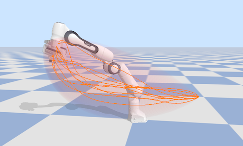
Computing the motion plan therefore entails optimizing these parameters with respect to an appropriate variational objective. Once optimized, in practice we can sample from the posterior using efficient sampling, that is, by first approximately sampling the prior $f(\cdot)$ using Fourier features, then transforming the sampled prior motion plans into posterior motion plans. This procedure allows us to draw random curves representing the posterior in a way that resolves the stochasticity once in advance per sample, after which we can evaluate and differentiate the motion plan at arbitrary time points without any additional sampling. Compared to prior work such as GPMP2 and its variants,⁵⁶⁷ we support general kernels and avoid relying on specialized techniques for stochastic differential equations, thereby enabling explicit control of motion plan smoothness properties. Additionally, in contrast with prior work,⁸ our formulation bypasses the need to use interpolation to evaluate the posterior in-between a set of pre-specified time points.

Following the framework of variational inference, the resulting variational posterior can be trained by solving the optimization problem

$$\min \mathbb{E}_{q(\boldsymbol{u})} \mathbb{E}_{p(\boldsymbol{f}\mid\boldsymbol{u})} \log p(\boldsymbol{e}\mid\boldsymbol{f}) - D_{\operatorname{KL}}(q(\boldsymbol{u})\mid\mid p(\boldsymbol{u}))$$

where $p(\boldsymbol{f}\mid\boldsymbol{u})$ is the log-likelihood term which in motion planning is used to encode soft constraints. To apply hard equality-based constraints, we use the fact that the variational posterior is Gaussian, and apply conditional probability to an appropriate set of $(z_j,u_j)$-pairs. We can also apply hard inequality-based constraints, such as joint constraints, and describe this further in the sequel.

This objective reveals Gaussian-process-based motion planning algorithms to be stochastic generalizations of optimization-based planners such as STOMP,⁹ CHOMP,¹⁰ and other variants: compared to these, the main difference is the presence of the Kullback–Leibler divergence, which prevents the posterior from collapsing to a single trajectory, thereby including uncertainty. For the log-likelihood, we use

$$p(\boldsymbol{e}\mid\boldsymbol{f}) = \exp\left(-\frac{1}{2} \left(\underset{\text{collision term}}{\undergroup{\left\|\operatorname{h}_\varepsilon(\operatorname{sdf}_s(\operatorname{k}_{\operatorname{fwd}}(\sigma(\boldsymbol{f}))))\right\|_{\mathbf\Sigma_{\operatorname{obs}}}^2}} + \underset{\text{soft constraint term}}{\undergroup{\left\|\operatorname{c}(\sigma(\boldsymbol{f}))\right\|^2_{\mathbf\Sigma_{\operatorname{c}}}}} \right)\right)$$

which, building on the approach used by GPMP2,⁶ works as follows. For the collision term, following CHOMP,¹⁰ we first approximate a robot by a set of spheres, and compute the signed distance field $\operatorname{sdf}_s$ for each sphere. This is done by composing the forward kinematics map $\operatorname{k}_{\operatorname{fwd}}$ with the constraint map $\sigma$ which enforces a set of box constraints to account for joint limits. Then, we compute the hinge loss $\operatorname{h}_\varepsilon(x) = \max(-x + \varepsilon, 0)$, where $\varepsilon$ is the safety distance parameter, and calculate its squared norm with respect to a diagonal scaling matrix $\mathbf\Sigma_{\operatorname{obs}}$ which determines the overall importance of avoiding collisions in the objective.

The soft constraint term, which can be used to encode desired behavior such as a grasping pose, is handled analogously. Compared to prior work,⁵⁶⁷⁸ one of the key differences is the introduction of $\sigma$, which guarantees that joint limits are respected without the need for clamping or other post-processing-based heuristics.

Experiments

Below, we provide a side-by-side comparison with our framework (vGPMP) and various baselines, on the UR10 and Franka robots. This comparison shows that, on these examples, vGPMP tends to result in higher mean clearance: the incorporation of uncertainty produce paths which are more conservative with respect to collision avoidance.

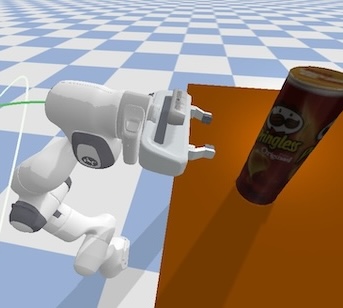
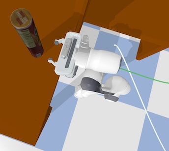
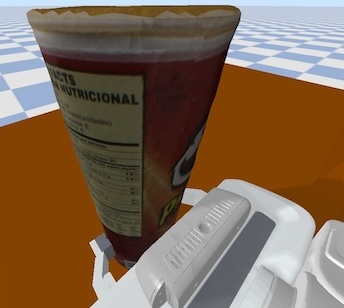
Next, we demonstrate that our framework can enable one to incorporate a grasping pose without further tuning or changing the underlying model assumptions. This amounts to adding appropriate terms to the soft constraints, and enables the Franka robot, in simulation, to pick up a can. Further adjustments to can be made to allow the robot to pick up the can and move it to desired places by conditioning end-effector joints to open and close at specific time steps.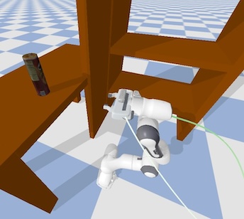

Finally we implement our approach on a real robot, via a demonstration of the Franka robot avoiding boxes. Here, our framework allows sampled paths to be computed at any required resolution without additional interpolation, enabling fine-grained control over smoothness. We also show a set of motion plans computed by the GPMP2 baseline,⁶ for comparison.

Conclusion

We present a unifying framework which simplifies motion planning with Gaussian processes by applying a formulation based on variational inference. Through the use of this inducing-point-based framework and pathwise conditioning, we support general kernels that provide explicit control over motion plan smoothness properties. Our computations are straightforward to implement, and avoid the need for interpolation, clipping, and other post-processing. The framework also connects Gaussian-process-based motion planning algorithms with optimization-based approaches. We evaluate the approach on different robots, showing that it accurately reaches target positions while avoiding obstacles, providing uncertainty, and increasing clearance compared to baselines. We demonstrate the approach on a real robot, executing a randomly sampled trajectory while avoiding obstacles.

References

M. Titsias. Variational learning of inducing variables in sparse Gaussian processes. AISTATS 2009.
J. Hensman, N. Fusi, and N. Lawrence. Gaussian Processes for Big Data. UAI 2013.
J. T. Wilson, V. Borovitskiy, A. Terenin, P. Mostowsky and M. P. Deisenroth. Efficiently Sampling Functions from Gaussian Process Posteriors. ICML 2020.
J. T. Wilson, V. Borovitskiy, A. Terenin, P. Mostowsky and M. P. Deisenroth. Pathwise Conditioning of Gaussian Processes. JMLR 2021.
M. Mukadam, X. Yan, and B. Boots. Gaussian process motion planning. ICRA 2016.
J. Dong, M. Mukadam, F. Dellaert, and B. Boots. Motion Planning as Probabilistic Inference using Gaussian Processes and Factor Graphs. RSS 2016.
M. Mukadam, J. Dong, X. Yan, F. Dellaert, and B. Boots. Continuous-time Gaussian Process Motion Planning via Probabilistic Inference. IJRR 2018.
H. Yu and Y. Chen. A Gaussian Variational Inference Approach to Motion Planning. RAL 2023.
M. Kalakrishnan, S. Chitta, E. Theodorou, P. Pastor, and S. Schaal. STOMP: Stochastic trajectory optimization for motion planning. ICRA 2011.
M. Zucker, N. Ratliff, A. Dragan, M. Pivtoraiko, M. Klingensmith, C. Dellin, J. A. Bagnell, and S. Srinivasa. CHOMP: Covariant Hamiltonian Optimization for Motion Planning. IJRR 2013.